Data Cleaning
This page is to prepare yourself for the fourth session of the DRA CashIM Series. It focuses on data cleaning in Excel.
Downloading data from kobo
To download data from kobotoolbox, please login at https://kobonew.ifrc.org and open your survey by clicking on “IM without Borders flooding registration form”. Then at the top, go to data and then to downloads at the left. Select “XLS” as export type and “Labels” as Value and header formats. Click on export. Then, after the download is processed, you can click download.

Data Cleaning in Excel
Navigation
There are multiple ways to navigate excel and select parts of your worksheet. The first option that you have is by using both the mouse and keyboard. By holding control on your keyboard and clicking on rows or columns, you can select them.
You can also use the keyboard-only. Then you can select columns by pressing control+space and rows by pressing shift+space. If you then hold shift, you can select multiple columns/rows by using the arrow keys.
Filter
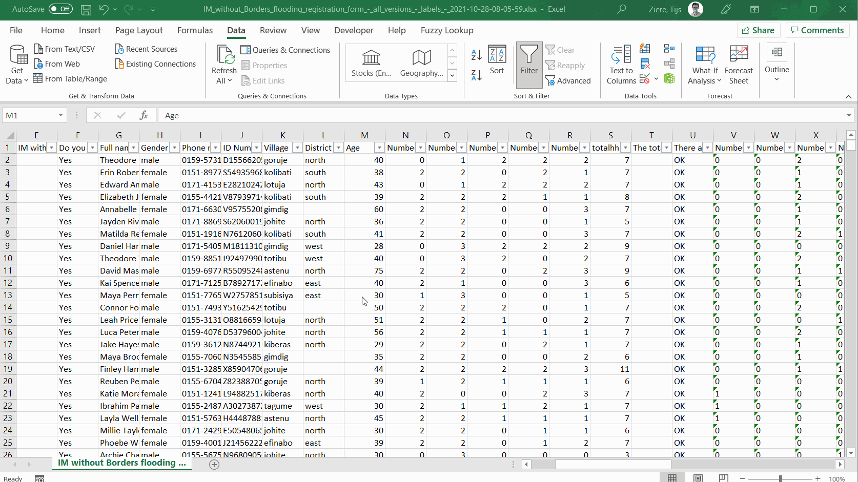
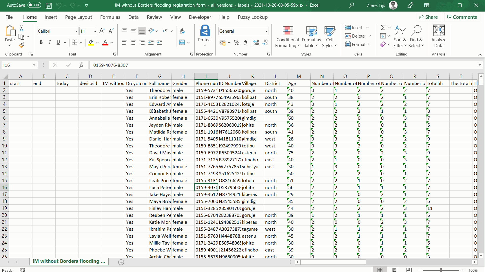
You can add filters by going to “Data” and then select “Filter”. Then you are able to filter your data based on the data you have in the different cells.
You can also add filters to sort your data, as vizualised below
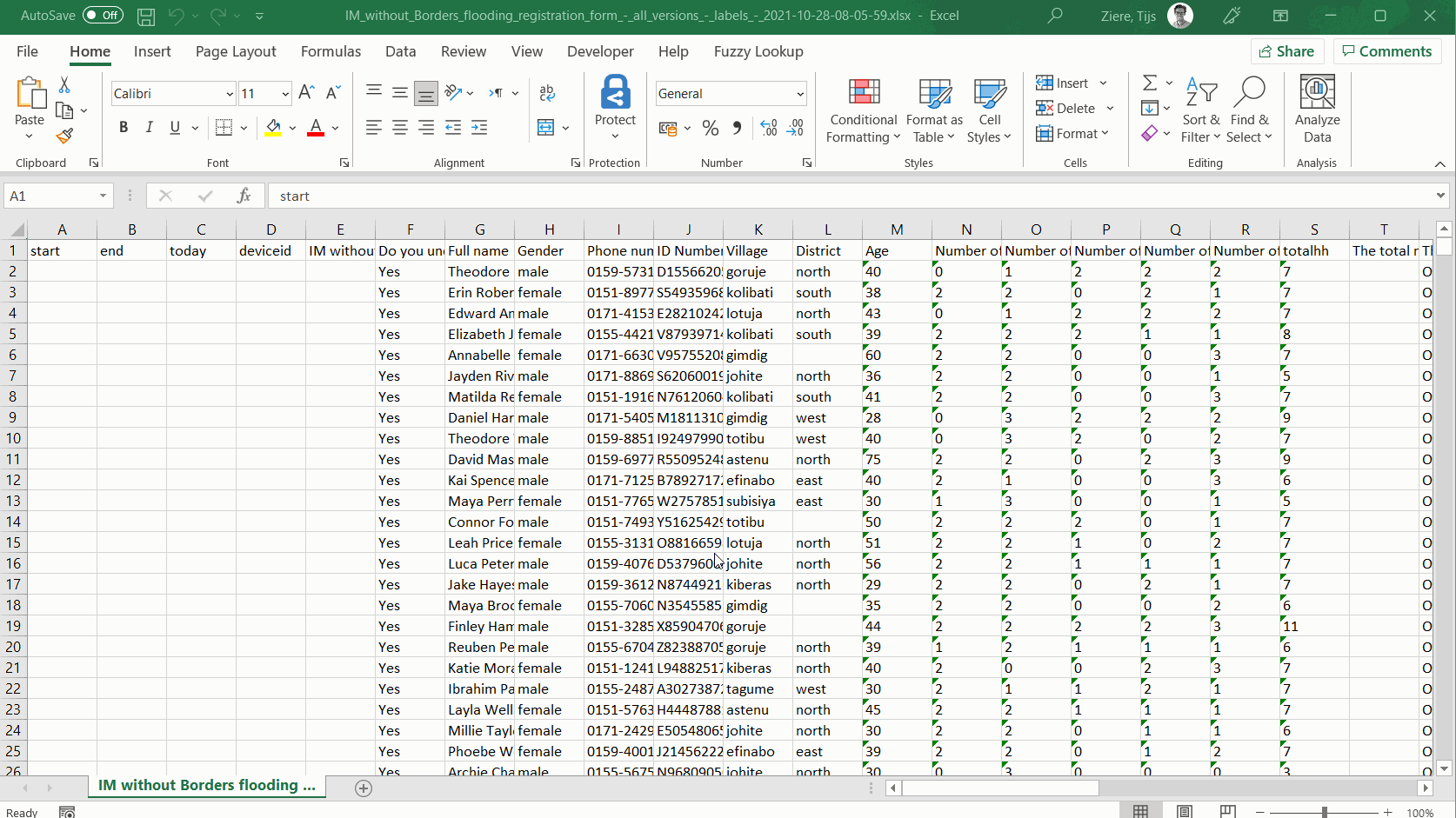
Go to special
The go-to-special function helps you select cell types. You can access it by clicking on “Home” at the top, then click on “Find & Select” and then click on “Go to special”. In the example below we will be selecting all the blank cells.
![]()
Replace
Find and replace is useful when you are changing large parts of your datasets. It is demonstrated in the video below. You can replace the first file Excel identifies by clicking “Replace” or replace all the values by “Replace All”.
Clear formatting
When you are done with your analysis, or you have other reasons to clear all your formatting, you can do so by going to “Home”, click the eraser button and then select “Clear formatting”.
![]()
Text functions (formulas) in Excel
Text functions are usefull to make sure all text is formatted in the same way. This helps with gettting a clear overview of the data, but also with automatic deduplication.
There are multiple text options that we will use:
- =TRIM(cell): Remove spaces from a text string except those between words: =TRIM()
- =PROPER(cell): First letter of each word capitalised
- =UPPER(cell): All letters uppercase
- =LOWER(cell): All letters lowercase
- =SUBSTITUTE(cell): substitute a value in a cell by something else
You can also combine these functions. For example: if you want to remove the leading and trailing spaces and capitalise each word in cell A1, you can use =PROPER(TRIM(A1)).
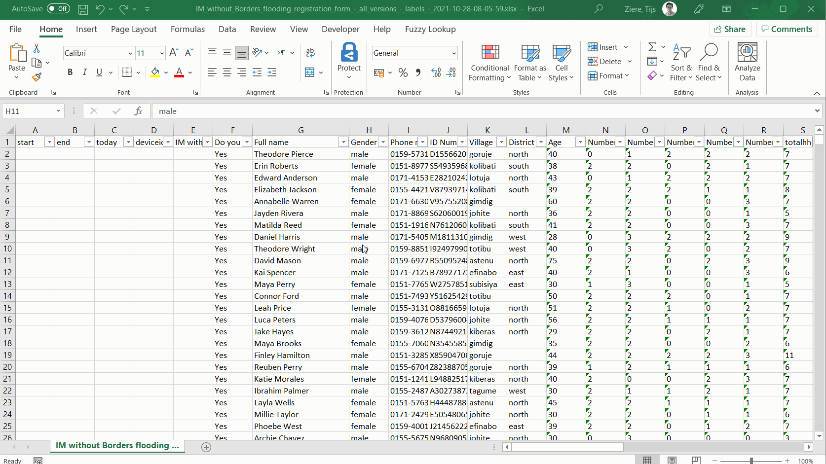
Text to columns
You can use text to columns if you want to split up text in a single cell into multiple columns. You can access the text to columns option by selecting the cells you want to split up, go to “Data”, and then click on “Text To Columns”. Then you have to select how you want to split up the cell, most often this is by a delimeter. Click next and specify the delimeter. This can by any of the default delimeters (in the video its a “;”), but you can also specify your custom delimeter. Then you click on next and you have the option to select a data-type for each column that is going to be created. You can also specify where you want your new data to be placed. If you then click finish, the data will be split in different columns, as is indicated by the video below.
Deduplication in Excel
There are mulitple ways to dedupe by using excel. For this part we will use conditional formatting on unique values (for example an ID Number, that is unique for every individual). If there are no unique we will create our own unique identifiers.
Conditional formatting (Hightlight Duplicates)
You can use conditional formatting in combination with Hightlight Duplicates, to identify doubles in your dataset. You can access highligth duplicates in “Home” and then click “Conditional Formatting”, select “Hightlight Cell Rules” and then select “Hightlight Duplicates”.
Create own unique identifiers
If your dataset does not include a unique identifier, you can try to create one yourself. You do this by combining different cells into one unique value. For example you can combine “firstname”, “lastname”, “village” and “date of birth”. The chance of somebody with the same name, that lives in the same village and has the same data of birth is very small. You can also combine this with the text functions for even better results.
You can do this with the concatenate function: =CONCAT(text1, text2, text3, …) or =text1&text2&text3&…
Then you can use hightlight duplicates to identify the duplicates.
Anomalies
Numeric Outliers
Check whether the range of values for each numeric question is as expected See range of values in the filter drop down, by sorting your table or by using formulas like MIN() and MAX().
Date Outliers
Check whether the range of values for each date question is as expected See range of values in the filter drop down, by sorting your table or by using formulas like MIN() and MAX().
Combining datasets
Sometimes you want to combine information from one dataset with information from another dataset. For example, if you did a first round of mobile data collection, but forgot to ask some questions. Then you go back into the field and ask the questions that you forgot to ask in the first round. After the second round of data collection, you want to combine the datasets into one. Below it is explained how to do this with the =VLOOKUP() function.
VLOOKUP for matching information with data.
VLOOKUP is structured as follows:
=VLOOKUP (lookup_value, table_array, col_index_num, [range_lookup]
lookup_value : value to look in 1st column
table_array : range of cells to search
col_index_num : column number
[range_lookup] : FALSE
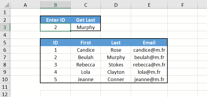
In the example below, we retrieve the last name of a person in another table. It uses the the third column (whitch is the last name), therefore it uses the value 3 in the formula.
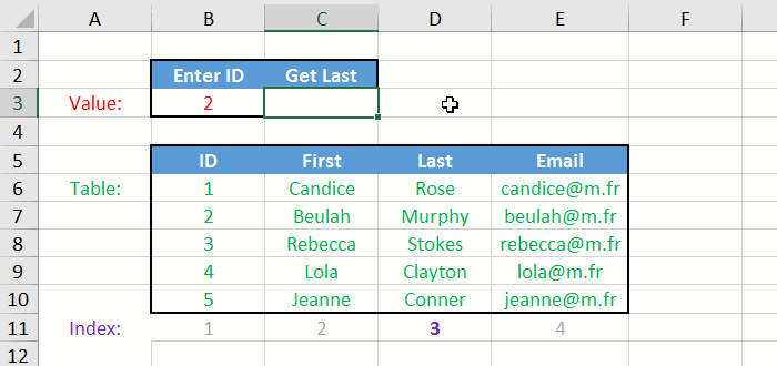
This is dynamic, so if you change the number in the other cell, the last name will also change:
More information can be found here